
t-tests
t-tests are used to determine whether the differences between the means of two normally distributed groups are statistically significant.
Independent t-test
Independent t-tests are used to assess the differences between the means of two separate, unrelated groups. Also known as 2-sample t-tests, independent sample t-tests, and student’s t-tests.
Example
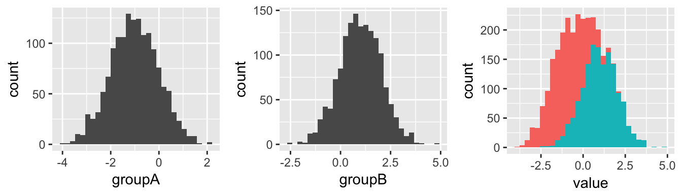
Consider the following 2 distributions.
Group A (left) has a normal distribution, with a mean of -1
Group B (center) has a normal distribution, with a mean of +1
When we plot them together (right), the difference is visible
##
##  Welch Two Sample t-test
##
## data:  listA and listB
## t = -53.878, df = 2992.2, p-value < 2.2e-16
## alternative hypothesis: true difference in means is not equal to 0
## 95 percent confidence interval:
##  -2.078726 -1.932740
## sample estimates:
## mean of x mean of y
## -1.014098  0.991635
Large t-value and a Small p-value <.01 = we accept the hypothesis that the means of list A and list B show statistically significant differences at a 99% confidence interval.
listA mean is estimated at approxiately -1 and listB mean is estimated at approximately 1.
The mean differences are listed as well showing the lowest & highest possible differences at 95% confidence.
Running Independent t-tests
If data are contained in 2 separate lists:
listA <- rnorm(1500, mean = -1)  #Produce list of random values w/ mean of -1 & normal distribtion
listB <- rnorm(1500, mean = 1) #Produce list of random values w/ mean of 1 & normal distribtion| listA | listB |
|---|---|
| 0.3331812 | 0.5523527 |
| -1.6772201 | 2.5600491 |
| 0.9139560 | 1.2009382 |
| -1.9383215 | 1.1982463 |
| -0.0096800 | 1.0137419 |
| -0.3920836 | 1.6985306 |
t.test syntax: t.test(variableA, variableB)
t.test(listA,listB) #If data are contained in two separate lists##
## Welch Two Sample t-test
##
## data: listA and listB
## t = -55.359, df = 2997.5, p-value < 2.2e-16
## alternative hypothesis: true difference in means is not equal to 0
## 95 percent confidence interval:
## -2.083782 -1.941222
## sample estimates:
## mean of x mean of y
## -1.0154567 0.9970449If data are contained in 1 dataset, distinguished by a binary grouping variable:
groupAB <- data.frame(listA, listB)%>%
           gather(groupAB)

kable(head(groupAB))| groupAB | value |
|---|---|
| listA | 0.3331812 |
| listA | -1.6772201 |
| listA | 0.9139560 |
| listA | -1.9383215 |
| listA | -0.0096800 |
| listA | -0.3920836 |
t.test syntax: t.test(continuous_var~binary_var, data=data)
t.test(value~groupAB, data=groupAB) ##
## Welch Two Sample t-test
##
## data: value by groupAB
## t = -55.359, df = 2997.5, p-value < 2.2e-16
## alternative hypothesis: true difference in means is not equal to 0
## 95 percent confidence interval:
## -2.083782 -1.941222
## sample estimates:
## mean in group listA mean in group listB
## -1.0154567 0.9970449Paired t-tests
If two sets of observations are made on the same subjets, in a before-and-after or other similar scenario, you can used a paired t-test
t.test syntax: t.test(continuous_var~binary_var, paried=TRUE, data=data)
t.test(value~groupAB, paired=TRUE, data=groupAB) ##
## Paired t-test
##
## data: value by groupAB
## t = -56.03, df = 1499, p-value < 2.2e-16
## alternative hypothesis: true difference in means is not equal to 0
## 95 percent confidence interval:
## -2.082957 -1.942046
## sample estimates:
## mean of the differences
## -2.012502Large t-value and a Small p-value <.01 = we accept the hypothesis that the means of listA and listB show statistically significant differences at a 99% confidence interval.
The mean of the differences: As the name implies, this shows the mean of the differences between groups. When comparing experimental results on the same group of subjects, this might be considered something of an effect size.